3. Watching a solar eclipse using an OOI moored echosounder#

Jupyter notebook accompanying the manuscript:

Echopype: A Python library for interoperable and scalable processing of ocean sonar data for biological information
Authors: Wu-Jung Lee, Emilio Mayorga, Landung Setiawan, Kavin Nguyen, Imran Majeed, Valentina Staneva

3.1. Introduction#

3.1.1. Goals#

Illustrate a common workflow for echosounder data conversion, calibration and use. This workflow leverages the standardization applied by echopype. and the power, ease of use and familiarity of libraries in the scientific Python ecosystem.
Demonstrate the ease to interoperate echosounder data with those from a different instrument in a single computing environment. Without echopype, additional wrangling across more than one software systems is needed to achieve the same visualization and comparison.

3.1.2. Description#

This notebook uses EK60 echosounder data from the U.S. Ocean Observatories Initiative (OOI) to illustrate a common workflow for data conversion, combination, calibration and analysis using echopype, as well as the data interoperability it enables. Without echopype, additional wrangling across more than one software systems is needed to achieve the same visualization and comparison.

We will use data from the OOI Oregon Offshore Cabled Shallow Profiler Mooring collected on August 20-21, 2017. This was the day before and of a solar eclipse, during which the reduced sunlight affected the regular diel vertical migration (DVM) patterns of marine life. This change was directly observed using the upward-looking echosounder mounted on this mooring platform that happened to be within the totality zone. The effect of the solar eclipse was clearly seen by aligning and comparing the echosounder observations with solar radiation data collected by the Bulk Meteorology Instrument Package located on the nearby Coastal Endurance Oregon Offshore Surface Mooring, also maintained by the OOI.

The data used are 19 .raw files with a total volume of approximately 1 GB. With echopype functionality, the raw data files hosted on the OOI Raw Data Archive (an HTTP server) are directly parsed and organized into a standardized representation following in the SONAR-netCDF4 v1.0 convention, and stored to the cloud-optimized Zarr format. The individual converted files are later combined into a single entity that can be easily explored and manipulated.

3.1.3. Outline#

Establish connection with the OOI Raw Data Archive and generate list of target EK60 .raw files
Process the archived raw files with echopype: convert and combine into a single quantity (an EchoData object) in a standardized format.
Obtain solar radiation data from an OOI Thredds server.
Plot the echosounder and solar radiation data together to visualize the zooplankton response to a solar eclipse.

3.1.4. Running the notebook#

This notebook can be run with a conda environment created using the conda environment file https://github.com/OSOceanAcoustics/echopype-examples/blob/main/binder/environment.yml. The notebook creates a directory ./exports/notebook3 and save all generated Zarr and netCDF files there.

3.1.5. Warning#

The compute_MVBS step in this notebook is not efficient for lazy-loaded data with echopype version 0.6.3. We plan to address this issue soon.

3.1.6. Note#

We encourage importing echopype as ep for consistency.

from pathlib import Path
import itertools as it
import datetime as dt
from dateutil import parser as dtparser

import fsspec
import xarray as xr
import matplotlib.pyplot as plt
import hvplot.xarray
import panel

import echopype as ep

import warnings
warnings.simplefilter("ignore", category=DeprecationWarning)

3.2. Establish connection with the OOI Raw Data Archive and generate list of target EK60 `.raw` files#

Access and inspect the publicly accessible OOI Raw Data Archive (an HTTP server) as if it were a local file system. This will be done through the Python fsspec file system and bytes storage interface. We will use fsspec.filesystem.glob (fs.glob) to generate a list of all EK60 .raw data files in the archive then filter on file names for target dates of interest.

fs = fsspec.filesystem('https')

ooi_raw_url = (
    "https://rawdata.oceanobservatories.org/files/"
    "CE04OSPS/PC01B/ZPLSCB102_10.33.10.143/2017/08"
)

Now let’s specify the range of dates we will be pulling data from. Note that the data filenames contain the time information but were recorded at UTC time.

def in_range(raw_file: str, start: dt.datetime, end: dt.datetime) -> bool:
    """Check if file url is in datetime range"""
    file_name = Path(raw_file).name
    file_datetime = dtparser.parse(file_name, fuzzy=True)
    return file_datetime >= start and file_datetime <= end

start_datetime = dt.datetime(2017, 8, 21, 7, 0)
end_datetime = dt.datetime(2017, 8, 22, 7, 0)

On the OOI Raw Data Archive, the monthly folder is further split to daily folders, so we can simply grab data from the desired days.

desired_day_urls = [f"{ooi_raw_url}/{day}" for day in range(start_datetime.day, end_datetime.day + 1)]

desired_day_urls

['https://rawdata.oceanobservatories.org/files/CE04OSPS/PC01B/ZPLSCB102_10.33.10.143/2017/08/21',
 'https://rawdata.oceanobservatories.org/files/CE04OSPS/PC01B/ZPLSCB102_10.33.10.143/2017/08/22']

Grab all raw files within daily folders by using the filesytem glob, just like the Linux glob.

all_raw_file_urls = it.chain.from_iterable([fs.glob(f"{day_url}/*.raw") for day_url in desired_day_urls])

desired_raw_file_urls = list(filter(
    lambda raw_file: in_range(
        raw_file, 
        start_datetime-dt.timedelta(hours=3),  # 3 hour buffer to select files
        end_datetime+dt.timedelta(hours=3)
    ), 
    all_raw_file_urls
))


print(f"There are {len(desired_raw_file_urls)} raw files within the specified datetime range.")

There are 19 raw files within the specified datetime range.

3.3. Process the archived raw files with `echopype`#

3.3.1. Examine the workflow by processing just one file#

Let’s first test the echopype workflow by converting and processing 1 file from the above list.

We will use ep.open_raw to directly read in a raw data file from the OOI HTTP server.

The type of sonar needs to be specified as an input argument. The echosounders on the OOI Regional Cabled Array are Simrad EK60 echosounder. All other uncabled echosounders are the Acoustic Zooplankton and Fisher Profiler (AZFP) manufacturered by ASL Environmental Sciences. Echopype supports both of these and other instruments (see echopype documentation for detail).

3.3.4. Quickly visualize the result#

The default xarray visualization functions are useful in getting a quick sense of the data.

First replace the channel dimension and coordinate with the frequency_nominal variable containing actual frequency values. Note that this step is possible only because there are no duplicated frequencies present.

ds_Sv = ep.consolidate.swap_dims_channel_frequency(ds_Sv)

ds_Sv.Sv.sel(frequency_nominal=200000).plot.pcolormesh(
    x='ping_time', cmap = 'jet', vmin=-80, vmax=-30
);

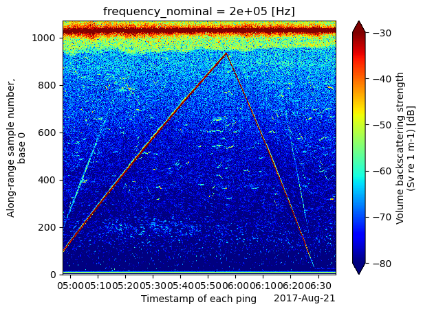
_images/ms_OOI_EK60_mooringtimeseries_35_0.png

Note that the vertical axis is range_sample. This is the bin (or sample) number as recorded in the data. A separate data variable in ds_Sv contains the physical range (echo_range) from the transducer in meters. echo_range has the same dimension as Sv and may not be uniform across all frequency channels or pings, depending on the echosounder setting during data collection.

3.3.5. Convert multiple files and combine into a single `EchoData` object#

Now that we verified that echopype does work for a single file, let’s proceed to process all sonar data from August 20-21, 2017.

First, convert all desired files from the OOI HTTP server to a local directory.

# Create a directory for all converted files
output_dpath = Path(base_dpath / 'convertallfiles')
output_dpath.mkdir(exist_ok=True)

%%time
for raw_file_url in desired_raw_file_urls:
    # Read and convert, resulting in echodata object
    ed = ep.open_raw(raw_file=raw_file_url, sonar_model='ek60', use_swap=True)
    ed.to_zarr(save_path=output_dpath, overwrite=True)

Then, assemble a list of EchoData object from the converted files. Note that by using chunks={}, the files are lazy-loaded and only metadata are read into memory, until more operations are executed.

ed_list = []
for converted_file in sorted(output_dpath.glob("*.zarr")):
#     ed_list.append(ep.open_converted(converted_file))
    ed_list.append(ep.open_converted(converted_file, chunks={}))

Combine all the opened files to a single EchoData object.

ed_combined = ep.combine_echodata(ed_list)

Below we can inspect this combined EchoData object just as before.

Expand the Provenance group to see how the filenames of all 19 files combined are stored in the coordinate variable echodata_filename, and many more data variables are added to retain information that was previously stored as attributes in the Provenance group of individual EchoData objects.

Expand the Sonar/Beam_group1 to see how data variables such as backscatter_r and angle_alongship contain chunked dask arrays (that are lazy-loadded), instead of regular numpy arrays (that are fully loaded into memory). This means that the computation needed to combine the EchoData objects are specified but not yet executed, which is why the previous line ran through so fast. This is also the mechanism that allows dask to perform its magic for out-of-core computation.

ed_combined

EchoData: standardized raw data from Internal Memory

Top-level: contains metadata about the SONAR-netCDF4 file format.

Environment: contains information relevant to acoustic propagation through water.

<xarray.Dataset> Size: 6MB
Dimensions:                 (channel: 3, time1: 109482)
Coordinates:
  * channel                 (channel) <U39 468B 'GPT  38 kHz 00907208dd13 5-1...
  * time1                   (time1) datetime64[ns] 876kB 2017-08-21T04:57:17....
Data variables:
    absorption_indicative   (channel, time1) float64 3MB dask.array<chunksize=(3, 5923), meta=np.ndarray>
    frequency_nominal       (channel) float64 24B dask.array<chunksize=(3,), meta=np.ndarray>
    sound_speed_indicative  (channel, time1) float64 3MB dask.array<chunksize=(3, 5923), meta=np.ndarray>

Platform: contains information about the platform on which the sonar is installed.

<xarray.Dataset> Size: 4MB
Dimensions:              (channel: 3, time1: 19, time2: 109478)
Coordinates:
  * time1                (time1) datetime64[ns] 152B 2017-08-21T04:57:17.3292...
  * channel              (channel) <U39 468B 'GPT  38 kHz 00907208dd13 5-1 OO...
  * time2                (time2) datetime64[ns] 876kB 2017-08-21T04:57:17.329...
Data variables: (12/20)
    MRU_offset_x         float64 8B nan
    MRU_offset_y         float64 8B nan
    MRU_offset_z         float64 8B nan
    MRU_rotation_x       float64 8B nan
    MRU_rotation_y       float64 8B nan
    MRU_rotation_z       float64 8B nan
    ...                   ...
    transducer_offset_y  (channel) float64 24B dask.array<chunksize=(3,), meta=np.ndarray>
    transducer_offset_z  (channel) float64 24B dask.array<chunksize=(3,), meta=np.ndarray>
    water_level          float64 8B 0.0
    pitch                (time2) float64 876kB dask.array<chunksize=(5923,), meta=np.ndarray>
    roll                 (time2) float64 876kB dask.array<chunksize=(5923,), meta=np.ndarray>
    vertical_offset      (time2) float64 876kB dask.array<chunksize=(5923,), meta=np.ndarray>
Attributes:
    platform_code_ICES:  
    platform_name:       
    platform_type:

NMEA: contains information specific to the NMEA protocol.

<xarray.Dataset> Size: 2kB
Dimensions:        (time1: 19)
Coordinates:
  * time1          (time1) datetime64[ns] 152B 2017-08-21T04:57:17.329287 ......
Data variables:
    NMEA_datagram  (time1) <U22 2kB dask.array<chunksize=(1,), meta=np.ndarray>
Attributes:
    description:  All NMEA sensor datagrams

Provenance: contains metadata about how the SONAR-netCDF4 version of the data were obtained.

<xarray.Dataset> Size: 27kB
Dimensions:                      (filenames: 19, echodata_filename: 19)
Coordinates:
  * filenames                    (filenames) int64 152B 0 1 2 3 ... 15 16 17 18
  * echodata_filename            (echodata_filename) <U26 2kB 'OOI-D20170821-...
Data variables: (12/24)
    source_filenames             (filenames) <U119 9kB dask.array<chunksize=(1,), meta=np.ndarray>
    conventions                  (echodata_filename) <U35 3kB 'CF-1.7, SONAR-...
    date_created                 (echodata_filename) <U20 2kB '2017-08-21T04:...
    keywords                     (echodata_filename) <U4 304B 'EK60' ... 'EK60'
    sonar_convention_authority   (echodata_filename) <U4 304B 'ICES' ... 'ICES'
    sonar_convention_name        (echodata_filename) <U13 988B 'SONAR-netCDF4...
    ...                           ...
    sonar_serial_number          (echodata_filename) <U1 76B '' '' '' ... '' ''
    sonar_software_name          (echodata_filename) <U4 304B 'ER60' ... 'ER60'
    sonar_software_version       (echodata_filename) <U5 380B '2.4.3' ... '2....
    sonar_type                   (echodata_filename) <U11 836B 'echosounder' ...
    beam_mode                    (echodata_filename) <U8 608B 'vertical' ... ...
    conversion_equation_t        (echodata_filename) <U6 456B 'type_3' ... 't...
Attributes:
    conversion_software_name:      echopype
    conversion_software_version:   0.8.4.dev58+gae911de
    conversion_time:               2024-04-24T14:55:05Z
    is_combined:                   True
    combination_software_name:     echopype
    combination_software_version:  0.8.4.dev58+gae911de
    combination_time:              2024-04-26T18:38:47Z

Sonar: contains sonar system metadata and sonar beam groups.

<xarray.Dataset> Size: 568B
Dimensions:           (beam_group: 1)
Coordinates:
  * beam_group        (beam_group) <U11 44B 'Beam_group1'
Data variables:
    beam_group_descr  (beam_group) <U131 524B dask.array<chunksize=(1,), meta=np.ndarray>
Attributes:
    sonar_manufacturer:      Simrad
    sonar_model:             EK60
    sonar_serial_number:     
    sonar_software_name:     ER60
    sonar_software_version:  2.4.3
    sonar_type:              echosounder

Beam_group1: contains backscatter power (uncalibrated) and other beam or channel-specific data, including split-beam angle data when they exist.

<xarray.Dataset> Size: 8GB
Dimensions:                        (channel: 3, ping_time: 109482,
                                    range_sample: 1072)
Coordinates:
  * channel                        (channel) <U39 468B 'GPT  38 kHz 00907208d...
  * ping_time                      (ping_time) datetime64[ns] 876kB 2017-08-2...
  * range_sample                   (range_sample) int64 9kB 0 1 2 ... 1070 1071
Data variables: (12/29)
    angle_alongship                (channel, ping_time, range_sample) float64 3GB dask.array<chunksize=(3, 3886, 1072), meta=np.ndarray>
    angle_athwartship              (channel, ping_time, range_sample) float64 3GB dask.array<chunksize=(3, 3886, 1072), meta=np.ndarray>
    angle_offset_alongship         (channel) float64 24B dask.array<chunksize=(3,), meta=np.ndarray>
    angle_offset_athwartship       (channel) float64 24B dask.array<chunksize=(3,), meta=np.ndarray>
    angle_sensitivity_alongship    (channel) float64 24B dask.array<chunksize=(3,), meta=np.ndarray>
    angle_sensitivity_athwartship  (channel) float64 24B dask.array<chunksize=(3,), meta=np.ndarray>
    ...                             ...
    transmit_bandwidth             (channel, ping_time) float64 3MB dask.array<chunksize=(3, 5923), meta=np.ndarray>
    transmit_duration_nominal      (channel, ping_time) float64 3MB dask.array<chunksize=(3, 5923), meta=np.ndarray>
    transmit_frequency_start       (channel) float64 24B dask.array<chunksize=(3,), meta=np.ndarray>
    transmit_frequency_stop        (channel) float64 24B dask.array<chunksize=(3,), meta=np.ndarray>
    transmit_power                 (channel, ping_time) float64 3MB dask.array<chunksize=(3, 5923), meta=np.ndarray>
    transmit_type                  <U2 8B 'CW'
Attributes:
    beam_mode:              vertical
    conversion_equation_t:  type_3

Vendor_specific: contains vendor-specific information about the sonar and the data.

<xarray.Dataset> Size: 892B
Dimensions:            (channel: 3, pulse_length_bin: 5)
Coordinates:
  * channel            (channel) <U39 468B 'GPT  38 kHz 00907208dd13 5-1 OOI....
  * pulse_length_bin   (pulse_length_bin) int64 40B 0 1 2 3 4
Data variables:
    frequency_nominal  (channel) float64 24B dask.array<chunksize=(3,), meta=np.ndarray>
    gain_correction    (channel, pulse_length_bin) float64 120B dask.array<chunksize=(3, 5), meta=np.ndarray>
    pulse_length       (channel, pulse_length_bin) float64 120B dask.array<chunksize=(3, 5), meta=np.ndarray>
    sa_correction      (channel, pulse_length_bin) float64 120B dask.array<chunksize=(3, 5), meta=np.ndarray>

3.3.7. Visualize MVBS interactively using `hvPlot`#

To visualize, invert the range axis since the echosounder is upward-looking from a platform at approximately 200 m water depth.

ds_MVBS = ds_MVBS.assign_coords(depth=("echo_range", ds_MVBS["echo_range"].values[::-1]))
ds_MVBS = ds_MVBS.swap_dims({'echo_range': 'depth'})  # set depth as data dimension

Then replace the channel dimension and coordinate with the frequency_nominal variable containing actual frequency values. Note that this step is possible only when there are no duplicated frequencies present.

ds_MVBS = ep.consolidate.swap_dims_channel_frequency(ds_MVBS)

ds_MVBS["Sv"].sel(frequency_nominal=200000).hvplot.image(
    x='ping_time', y='depth', 
    color='Sv', rasterize=True, 
    cmap='jet', clim=(-80, -30),
    xlabel='Time (UTC)',
    ylabel='Depth (m)',
).options(width=800, invert_yaxis=True)

/Users/wujung/miniconda3/envs/echopype_examples_20240424/lib/python3.10/site-packages/dask/dataframe/__init__.py:31: FutureWarning: 
Dask dataframe query planning is disabled because dask-expr is not installed.

You can install it with `pip install dask[dataframe]` or `conda install dask`.
This will raise in a future version.

  warnings.warn(msg, FutureWarning)
OMP: Info #276: omp_set_nested routine deprecated, please use omp_set_max_active_levels instead.

Note that the reflection from the sea surface shows up at a location below the depth of 0 m. This is because we have not corrected for the actual depth of the platform on which the echosounder is mounted, and the actual sound speed at the time of data collection (which is related to the calculated range) could also be different from the user-defined sound speed stored in the data file. More accurate platform depth information can be obtained using data from the CTD collocated on the moored platform.

3.5. Combine sonar observation with solar radiation measurements#

We can finally put everything together and figure out the impact of the eclipse-driven reduction in sunlight on marine zooplankton!

metbk_plot = metbk_ds.hvplot.line(
    x='time', y='shortwave_irradiance', responsive=True,
).options(width=800, height=120, logy=True, xlim=(start_datetime, end_datetime))

mvbs_plot = ds_MVBS["Sv"].sel(frequency_nominal=200000, ping_time=slice(start_datetime, end_datetime)).hvplot.image(
    x='ping_time', y='depth', 
    color='Sv', rasterize=True, 
    cmap='jet', clim=(-80, -30),
    xlabel='Time (UTC)',
    ylabel='Depth (m)'
).options(width=800, invert_yaxis=True)

(metbk_plot + mvbs_plot).cols(1)

Look how the dip at solar radiation reading matches exactly with the upwarding moving “blip” at UTC 17:21, August 22, 2017 (local time 10:22 AM). During the solar eclipse, the animals were fooled by the temporary mask of the sun and thought it’s getting dark as at dusk!

3.6. Package versions#

import datetime
print(f"echopype: {ep.__version__}, xarray: {xr.__version__}, fsspec: {fsspec.__version__}, "
      f"hvplot: {hvplot.__version__}")

print(f"\n{datetime.datetime.utcnow()} +00:00")

echopype: 0.8.4.dev58+gae911de, xarray: 2024.3.0, fsspec: 2024.3.1, hvplot: 0.9.2

2024-04-26 18:40:44.953619 +00:00

Echopype Examples

Watching a solar eclipse using an OOI moored echosounder

Contents

3. Watching a solar eclipse using an OOI moored echosounder#

3.1. Introduction#

3.1.1. Goals#

3.1.2. Description#

3.1.3. Outline#

3.1.4. Running the notebook#

3.1.5. Warning#

3.1.6. Note#

3.2. Establish connection with the OOI Raw Data Archive and generate list of target EK60 `.raw` files#

3.3. Process the archived raw files with `echopype`#

3.3.1. Examine the workflow by processing just one file#

3.3.2. Converting from raw data files to a standardized data format#

3.3.3. Basic echo processing#

3.3.4. Quickly visualize the result#

3.3.5. Convert multiple files and combine into a single `EchoData` object#

3.3.6. Calibrate the combined `EchoData` and visualize the mean Sv#

3.3.7. Visualize MVBS interactively using `hvPlot`#

3.4. Obtain solar radiation data from an OOI THREDDS server#

3.5. Combine sonar observation with solar radiation measurements#

3.6. Package versions#

Echopype Examples

Watching a solar eclipse using an OOI moored echosounder

Contents

3. Watching a solar eclipse using an OOI moored echosounder#

3.1. Introduction#

3.1.1. Goals#

3.1.2. Description#

3.1.3. Outline#

3.1.4. Running the notebook#

3.1.5. Warning#

3.1.6. Note#

3.2. Establish connection with the OOI Raw Data Archive and generate list of target EK60 .raw files#

3.3. Process the archived raw files with echopype#

3.3.1. Examine the workflow by processing just one file#

3.3.2. Converting from raw data files to a standardized data format#

3.3.3. Basic echo processing#

3.3.4. Quickly visualize the result#

3.3.5. Convert multiple files and combine into a single EchoData object#

3.3.6. Calibrate the combined EchoData and visualize the mean Sv#

3.3.7. Visualize MVBS interactively using hvPlot#

3.4. Obtain solar radiation data from an OOI THREDDS server#

3.5. Combine sonar observation with solar radiation measurements#

3.6. Package versions#

3.2. Establish connection with the OOI Raw Data Archive and generate list of target EK60 `.raw` files#

3.3. Process the archived raw files with `echopype`#

3.3.5. Convert multiple files and combine into a single `EchoData` object#

3.3.6. Calibrate the combined `EchoData` and visualize the mean Sv#

3.3.7. Visualize MVBS interactively using `hvPlot`#